18 贝叶斯统计推断

library(tidyverse)

── Attaching packages ─────────────────────────────────────── tidyverse 1.3.2 ──
✔ ggplot2 3.4.0     ✔ purrr   1.0.1
✔ tibble  3.1.8     ✔ dplyr   1.1.0
✔ tidyr   1.3.0     ✔ stringr 1.5.0
✔ readr   2.1.4     ✔ forcats 0.5.2
── Conflicts ────────────────────────────────────────── tidyverse_conflicts() ──
✖ dplyr::filter() masks stats::filter()
✖ dplyr::lag()    masks stats::lag()

library(tidybayes)
library(rstan)

Loading required package: StanHeaders
rstan (Version 2.21.7, GitRev: 2e1f913d3ca3)
For execution on a local, multicore CPU with excess RAM we recommend calling
options(mc.cores = parallel::detectCores()).
To avoid recompilation of unchanged Stan programs, we recommend calling
rstan_options(auto_write = TRUE)

Attaching package: 'rstan'

The following object is masked from 'package:tidyr':

    extract

library(brms)

Loading required package: Rcpp
Loading 'brms' package (version 2.18.0). Useful instructions
can be found by typing help('brms'). A more detailed introduction
to the package is available through vignette('brms_overview').

Attaching package: 'brms'

The following object is masked from 'package:rstan':

    loo

The following objects are masked from 'package:tidybayes':

    dstudent_t, pstudent_t, qstudent_t, rstudent_t

The following object is masked from 'package:stats':

    ar

rstan_options(auto_write = TRUE)
options(mc.cores = parallel::detectCores())

18.1 基本概念

贝叶斯定理

\[\underbrace{\Pr(\text{parameters} | \text{data})}_{\text{posterior}} = \frac{\overbrace{\Pr(\text{data} | \text{parameters})}^{\text{likelihood}} \overbrace{\Pr(\text{parameters})}^{\text{prior}}}{\underbrace{\Pr(\text{data})}_{evidence}}\] 这个量实际上贝叶斯定理中的后验概率分布(posterior distribution)

18.2 推断

注意到，我们的数据只是样本，不代表全体分布。我们只有通过样本去推断全体分布情况。

18.3 案例分析

icecream <- data.frame(
  temp = c( 11.9, 14.2, 15.2, 16.4, 17.2, 18.1, 
         18.5, 19.4, 22.1, 22.6, 23.4, 25.1),
  units = c( 185L, 215L, 332L, 325L, 408L, 421L, 
          406L, 412L, 522L, 445L, 544L, 614L)
  )
icecream

   temp units
1  11.9   185
2  14.2   215
3  15.2   332
4  16.4   325
5  17.2   408
6  18.1   421
7  18.5   406
8  19.4   412
9  22.1   522
10 22.6   445
11 23.4   544
12 25.1   614

icecream %>% 
  ggplot(aes(temp, units)) + 
  geom_point()

icecream%>%
  ggplot(aes(units))+
  geom_density()

18.3.1 线性回归函数`lm()`

fit_lm <- lm(units ~ 1+temp,data = icecream)
summary(fit_lm)


Call:
lm(formula = units ~ 1 + temp, data = icecream)

Residuals:
    Min      1Q  Median      3Q     Max 
-75.512 -12.566   4.133  22.236  49.963 

Coefficients:
            Estimate Std. Error t value Pr(>|t|)    
(Intercept) -159.474     54.641  -2.919   0.0153 *  
temp          30.088      2.866  10.499 1.02e-06 ***
---
Signif. codes:  0 '***' 0.001 '**' 0.01 '*' 0.05 '.' 0.1 ' ' 1

Residual standard error: 38.13 on 10 degrees of freedom
Multiple R-squared:  0.9168,    Adjusted R-squared:  0.9085 
F-statistic: 110.2 on 1 and 10 DF,  p-value: 1.016e-06

confint(fit_lm, level = 0.95)

                 2.5 %    97.5 %
(Intercept) -281.22128 -37.72702
temp          23.70223  36.47350

coef <- summary(fit_lm)$coefficients[2, 1] 
err  <- summary(fit_lm)$coefficients[2, 2]

coef + c(-1,1)*err*qt(0.975,  nrow(icecream) - 2)

[1] 23.70223 36.47350

在计量中，线性模型的几个基本假设： - 线性 - 各个观测值满足iid - 误差项满足正态分布 - 所有误差项有同方差

stan_program <- "
data {
  int<lower=0> N;
  vector[N] y;
  vector[N] x;
}
parameters {
  real alpha;
  real beta;
  real<lower=0> sigma;
}
model {
  y ~ normal(alpha + beta * x, sigma);
  
  alpha  ~ normal(0, 10);
  beta   ~ normal(0, 10);
  sigma  ~ exponential(1);
}

"

library("rstan")

library("loo")

This is loo version 2.5.1

- Online documentation and vignettes at mc-stan.org/loo

- As of v2.0.0 loo defaults to 1 core but we recommend using as many as possible. Use the 'cores' argument or set options(mc.cores = NUM_CORES) for an entire session.


Attaching package: 'loo'

The following object is masked from 'package:rstan':

    loo

seed <- 9547
set.seed(seed)

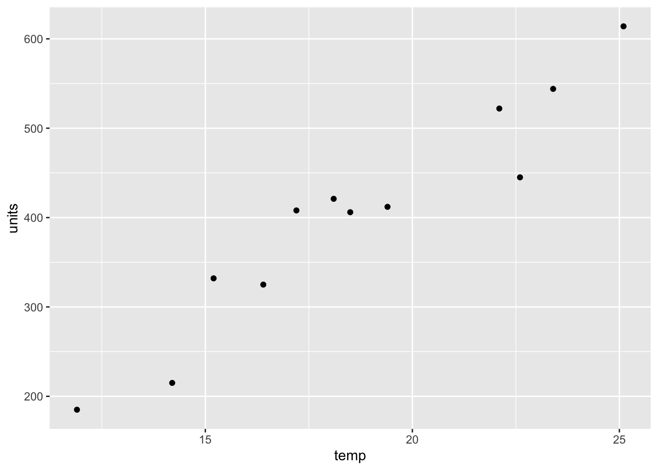
stan_data <- list(
   N = nrow(icecream),
   x = icecream$temp, 
   y = icecream$units
  )
fit_normal <- stan(model_code = stan_program, data = stan_data)

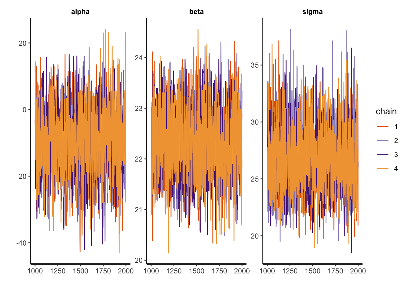
Traceplot图

traceplot(fit_normal)

1 主观概率与不确定性

不确定的高低用概率来表示，必然包含人们的主观判断；

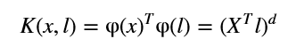
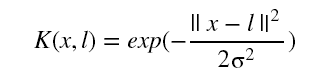
核函数：https://en.wikipedia.org/wiki/Positive-definite_kernel是作为一种运算技巧(Kernel Function)若$\phi(x)$是$x$在高维的映射，那么我们定义核函数为： \[ K(x,l)=\phi(x)^T\phi(l) \] 类似的，如果特征维度为 n ，映射的阶数为 d，那我们可以得到的结果是：

降低了时间复杂度；

kernel function 的判定：

根据Mercer定理，任何半正定的函数都可以作为kernel function

18.3.2 常用的kernel function:高斯核函数

1img

高斯核函数可以将原始的特征空间映射到无穷维的特征空间。对于样本$\{x(1),x(2),x(3),\cdots,x(m)\}$，$l$的取值是所有的$X$

18.3.3 极大似然估计

考虑一个M类问题：第m类别的数据子集$X_m$对应的概率密度函数是$p(x|\omega_m)$

需要确定数据的概率分布，需要知道概率分布函数的形式和参数，一个基本假设，概率分布的形式已知，比如满足高斯分布，那么似然函数就可以以参数$\theta$来表示，若是高斯分布，参数$\mu_i$和$\sigma^2$，即$\theta=(\mu_i,\sigma^2)$

18.3.4 渐近无偏

极大似然是渐近无偏的： \[ \lim_{N\to0}E[\hat \theta_{ML}]=\theta_0 \] 这里认为的估计值$\hat \theta$本身就是一个随机变量，其均值就是未知参数的真实值，就是渐近无偏；

18.3.5 渐近一致

即：$\lim_{n\to \infty}prob\{||\hat \theta_{ML}-\theta_0\leq \epsilon\}=1$满足一致性就不会形成震荡；

18.3.6 最大后验估计

最大似然估计中，将$\theta$看作未知参数，而最大后验估计中，将$$看作一个随机变量，并在已知样本中估计参数$$

https://bookdown.org/wangminjie/R4DS/bayesian-glm-logistic-binomial.html

18.4 理解线性回归

对于线性回归：可以从频率学派和贝叶斯学派来理解：

频率学派中，weight value $\omega$是一个未知的常数，因此可以将其转化为一个最优化问题，对其进行点估计，就是2-范数最小化：

18.5 条件分布$p(\omega|Data)$

根据贝叶斯原理，后验概率可以由先验概率和似然概率得到：