8  EDA

8.1 什么是EDA

探索性数据分析：Exporatory data analysis，是对于各种知识的应用。

8.2 导入数据

library(tidyverse)

── Attaching packages ─────────────────────────────────────── tidyverse 1.3.2 ──
✔ ggplot2 3.4.0     ✔ purrr   1.0.1
✔ tibble  3.1.8     ✔ dplyr   1.1.0
✔ tidyr   1.3.0     ✔ stringr 1.5.0
✔ readr   2.1.4     ✔ forcats 0.5.2
── Conflicts ────────────────────────────────────────── tidyverse_conflicts() ──
✖ dplyr::filter() masks stats::filter()
✖ dplyr::lag()    masks stats::lag()

library(lubridate)

Loading required package: timechange

Attaching package: 'lubridate'

The following objects are masked from 'package:base':

    date, intersect, setdiff, union

df<-read_csv('nobel_prize_by_winner.csv')

Rows: 972 Columns: 20
── Column specification ────────────────────────────────────────────────────────
Delimiter: ","
chr (17): firstname, surname, born, died, bornCountry, bornCountryCode, born...
dbl  (3): id, year, share

ℹ Use `spec()` to retrieve the full column specification for this data.
ℹ Specify the column types or set `show_col_types = FALSE` to quiet this message.

df

# A tibble: 972 × 20
      id firstname   surname born  died  bornC…¹ bornC…² bornC…³ diedC…⁴ diedC…⁵
   <dbl> <chr>       <chr>   <chr> <chr> <chr>   <chr>   <chr>   <chr>   <chr>  
 1   846 Elinor      Ostrom  8/7/… 6/12… USA     US      "Los A… USA     US     
 2   846 Elinor      Ostrom  8/7/… 6/12… USA     US      "Los A… USA     US     
 3   783 Wangari Mu… Maathai 4/1/… 9/25… Kenya   KE      "Nyeri" Kenya   KE     
 4   230 Dorothy Cr… Hodgkin 5/12… 7/29… Egypt   EG      "Cairo" United… GB     
 5   918 Youyou      Tu      12/3… 0000… China   CN      "Zheji… <NA>    <NA>   
 6   428 Barbara     McClin… 6/16… 9/2/… USA     US      "Hartf… USA     US     
 7   773 Shirin      Ebadi   6/21… 0000… Iran    IR      "Hamad… <NA>    <NA>   
 8   597 Grazia      Deledda 09/2… 8/15… Italy   IT      "Nuoro… Italy   IT     
 9   615 Gabriela    Mistral 04/0… 1/10… Chile   CL      "Vicu_… USA     US     
10   782 Elfriede    Jelinek 10/2… 0000… Austria AT      "M\xf4… <NA>    <NA>   
# … with 962 more rows, 10 more variables: diedCity <chr>, gender <chr>,
#   year <dbl>, category <chr>, overallMotivation <chr>, share <dbl>,
#   motivation <chr>, name <chr>, city <chr>, country <chr>, and abbreviated
#   variable names ¹​bornCountry, ²​bornCountryCode, ³​bornCity, ⁴​diedCountry,
#   ⁵​diedCountryCode

colnames(df)

 [1] "id"                "firstname"         "surname"          
 [4] "born"              "died"              "bornCountry"      
 [7] "bornCountryCode"   "bornCity"          "diedCountry"      
[10] "diedCountryCode"   "diedCity"          "gender"           
[13] "year"              "category"          "overallMotivation"
[16] "share"             "motivation"        "name"             
[19] "city"              "country"          

在这个数据中，发现是存在重复数据行的现象，由此我们使用函数distinct来是被和保留重复数据，id来识别重复数据，.keep_all来保留所有的变量。

df<-df%>%
    distinct(id,.keep_all= TRUE)
dim(df)

[1] 907  20

删去了70个重复数据。

8.2.0.1 缺失数据

df %>% map_df(~sum(is.na(.)))

# A tibble: 1 × 20
     id firstname surname  born  died bornCoun…¹ bornC…² bornC…³ diedC…⁴ diedC…⁵
  <int>     <int>   <int> <int> <int>      <int>   <int>   <int>   <int>   <int>
1     0         6      33    23    23         29      29      31     333     334
# … with 10 more variables: diedCity <int>, gender <int>, year <int>,
#   category <int>, overallMotivation <int>, share <int>, motivation <int>,
#   name <int>, city <int>, country <int>, and abbreviated variable names
#   ¹​bornCountry, ²​bornCountryCode, ³​bornCity, ⁴​diedCountry, ⁵​diedCountryCode

该数据中存在一些缺失的情况，包括名字、姓氏、出生国家等等。根据我们所探索数据的需要来分别使用不同的方法来进行处理。

8.3 所要探究的问题

8.3.1 获得诺贝尔国家数

df%>%
  drop_na(country)%>%
  count(country,sort = T)

# A tibble: 29 × 2
   country                         n
   <chr>                       <int>
 1 USA                           339
 2 United Kingdom                 89
 3 Germany                        43
 4 France                         34
 5 Federal Republic of Germany    23
 6 Switzerland                    21
 7 Sweden                         17
 8 Japan                          16
 9 the Netherlands                11
10 Denmark                         9
# … with 19 more rows

8.3.2 获奖类别

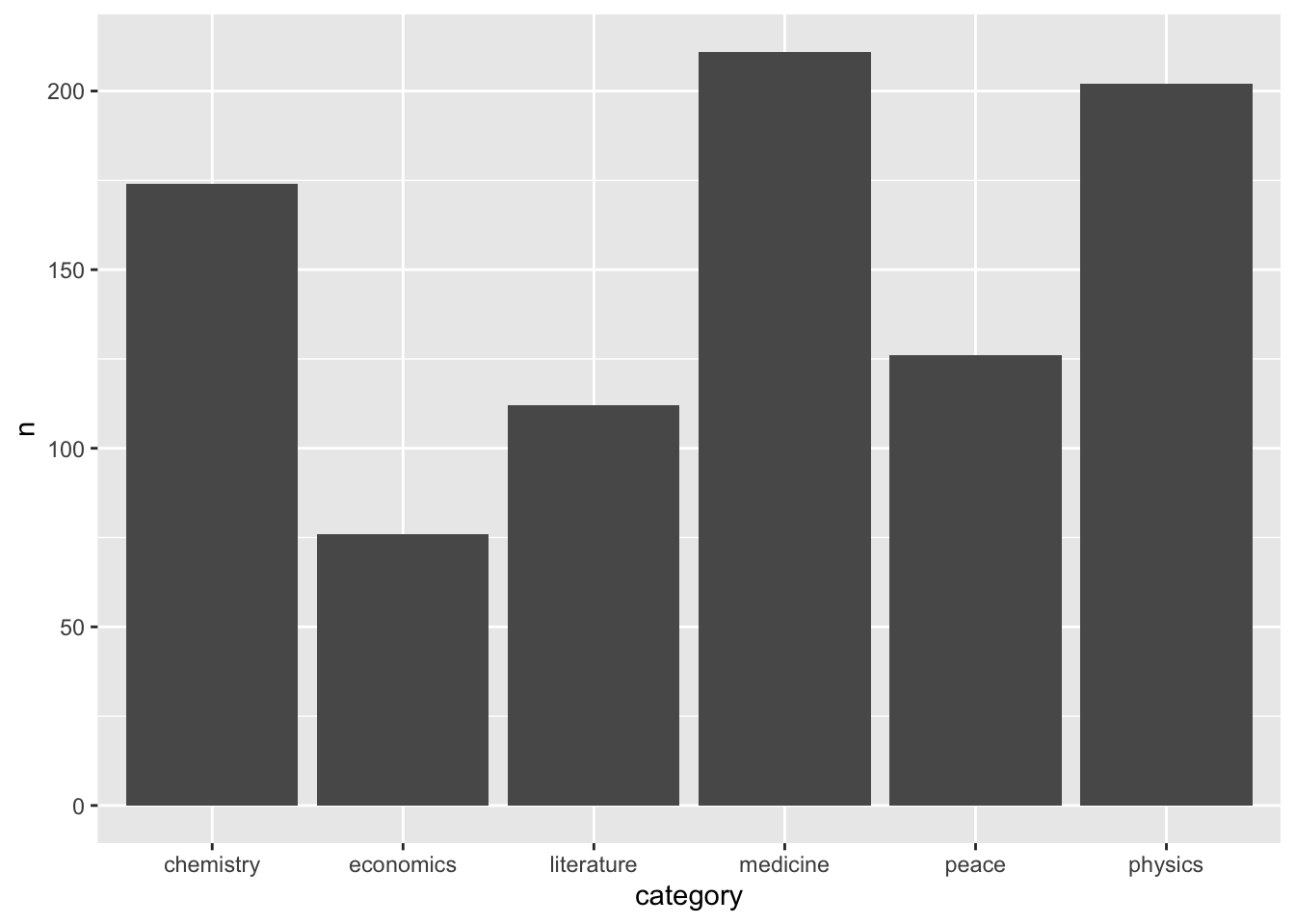
df %>% 
  count(category)

# A tibble: 7 × 2
  category       n
  <chr>      <int>
1 chemistry    174
2 economics     76
3 literature   112
4 medicine     211
5 peace        126
6 physics      202
7 <NA>           6

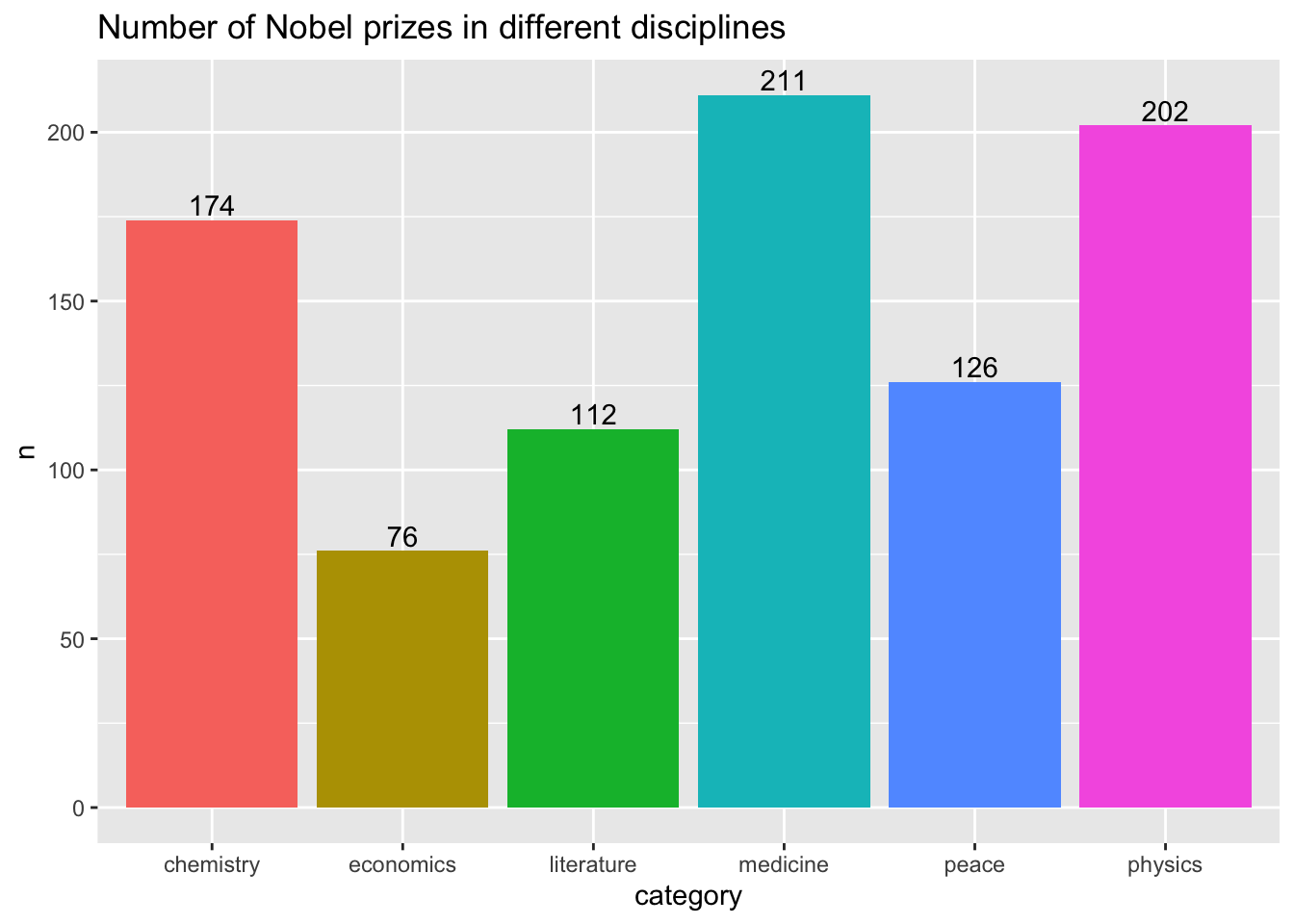
df %>%
  drop_na(category)%>%
  count(category)%>%
  ggplot(aes(x = category,y = n))+
  geom_col()

当然可以进一步调整图像：

df %>%
  drop_na(category)%>%
  count(category)%>%
  ggplot(aes(x = category,y = n,fill = category))+
  geom_col()+
  geom_text(aes(label=n),vjust=-0.25)+
  labs(title = "Number of Nobel prizes in different disciplines") +
  theme(legend.position = "none")

显然经济学是最少的，因为进入的晚一些，另一方面可能学科发展上，可能经常是一个人一次拿一个炸药奖，其他学科需要进行合作，所探究的问题是相同领域的。

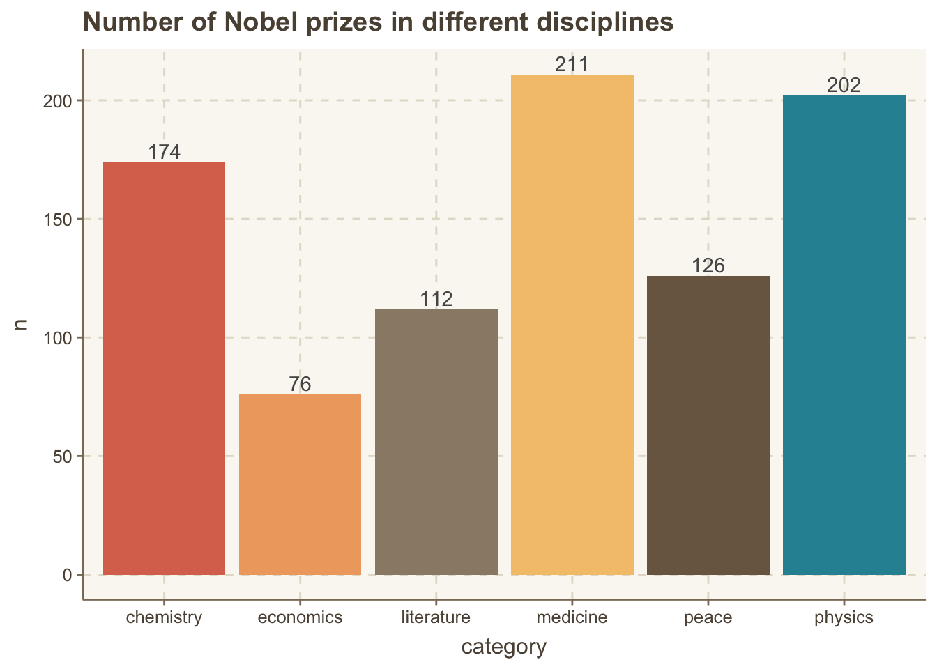
library(ggthemr)
ggthemr("dust")
df %>%
  drop_na(category)%>%
  count(category)%>%
  ggplot(aes(x = category,y = n,fill = category))+
  geom_col()+
  geom_text(aes(label=n),vjust=-0.25)+
  labs(title = "Number of Nobel prizes in different disciplines") +
  theme(legend.position = "none")

df %>%
  dplyr::filter(bornCountry == "China") %>%
  dplyr::select(firstname,surname, year, category)

# A tibble: 11 × 4
   firstname        surname   year category  
   <chr>            <chr>    <dbl> <chr>     
 1 Youyou           Tu        2015 medicine  
 2 Gao              Xingjian  2000 literature
 3 Charles Kuen     Kao       2009 physics   
 4 Liu              Xiaobo    2010 peace     
 5 Ei-ichi          Negishi   2010 chemistry 
 6 Edmond H.        Fischer   1992 medicine  
 7 Daniel C.        Tsui      1998 physics   
 8 Tsung-Dao (T.D.) Lee       1957 physics   
 9 Chen Ning        Yang      1957 physics   
10 Walter Houser    Brattain  1956 physics   
11 Mo               Yan       2012 literature

看到这份名单还是有一些感慨的。

df %>% count(surname, sort = T)

# A tibble: 831 × 2
   surname         n
   <chr>       <int>
 1  <NA>          33
 2 "Fischer"       4
 3 "Smith"         4
 4 "Wilson"        4
 5 "Lee"           3
 6 "Lewis"         3
 7 "M\xf4ller"     3
 8 "Anderson"      2
 9 "Bloch"         2
10 "Bohr"          2
# … with 821 more rows

df<-df%>%
  mutate(birthyear=year(strptime(df$born,format ="%m/%d/%Y")))

library(lubridate)
nobel_winner<-df%>%
  distinct_at(vars(surname,firstname, year, category), .keep_all = TRUE) %>%
  mutate(
    decade = 10 * (year%/%10),
    prize_age = year-birthyear,
    full_name = paste(surname,firstname)
)
head(nobel_winner)

# A tibble: 6 × 24
     id firstname    surname born  died  bornC…¹ bornC…² bornC…³ diedC…⁴ diedC…⁵
  <dbl> <chr>        <chr>   <chr> <chr> <chr>   <chr>   <chr>   <chr>   <chr>  
1   846 Elinor       Ostrom  8/7/… 6/12… USA     US      Los An… USA     US     
2   783 Wangari Muta Maathai 4/1/… 9/25… Kenya   KE      Nyeri   Kenya   KE     
3   230 Dorothy Cro… Hodgkin 5/12… 7/29… Egypt   EG      Cairo   United… GB     
4   918 Youyou       Tu      12/3… 0000… China   CN      Zhejia… <NA>    <NA>   
5   428 Barbara      McClin… 6/16… 9/2/… USA     US      Hartfo… USA     US     
6   773 Shirin       Ebadi   6/21… 0000… Iran    IR      Hamadan <NA>    <NA>   
# … with 14 more variables: diedCity <chr>, gender <chr>, year <dbl>,
#   category <chr>, overallMotivation <chr>, share <dbl>, motivation <chr>,
#   name <chr>, city <chr>, country <chr>, birthyear <dbl>, decade <dbl>,
#   prize_age <dbl>, full_name <chr>, and abbreviated variable names
#   ¹​bornCountry, ²​bornCountryCode, ³​bornCity, ⁴​diedCountry, ⁵​diedCountryCode

nobel_winner %>%
  group_by(full_name) %>%
  mutate(
    number_prize = n(),
    number_cateory = n_distinct(category)
  ) %>%
  arrange(desc(number_prize), full_name) %>%
  dplyr::filter(number_cateory == 2)

# A tibble: 0 × 26
# Groups:   full_name [0]
# … with 26 variables: id <dbl>, firstname <chr>, surname <chr>, born <chr>,
#   died <chr>, bornCountry <chr>, bornCountryCode <chr>, bornCity <chr>,
#   diedCountry <chr>, diedCountryCode <chr>, diedCity <chr>, gender <chr>,
#   year <dbl>, category <chr>, overallMotivation <chr>, share <dbl>,
#   motivation <chr>, name <chr>, city <chr>, country <chr>, birthyear <dbl>,
#   decade <dbl>, prize_age <dbl>, full_name <chr>, number_prize <int>,
#   number_cateory <int>

nobel_winner %>%
  count(prize_age)%>%
  drop_na()%>%
  ggplot(aes(x = prize_age, y = n)) +
  geom_col()

nobel_winner %>%
  group_by(category) %>%
  summarise(mean_prize_age = mean(prize_age, na.rm = T))

# A tibble: 7 × 2
  category   mean_prize_age
  <chr>               <dbl>
1 chemistry            57.8
2 economics            67.2
3 literature           64.6
4 medicine             57.9
5 peace                61.4
6 physics              55.2
7 <NA>                NaN  

nobel_winner %>%
  mutate(category = fct_reorder(category, prize_age, median, na.rm = TRUE)) %>%
  ggplot(aes(category, prize_age)) +
  geom_point() +
  geom_boxplot() +
  coord_flip()

Warning: Removed 36 rows containing non-finite values (`stat_boxplot()`).

Warning: Removed 36 rows containing missing values (`geom_point()`).

head(nobel_winner)

# A tibble: 6 × 24
     id firstname    surname born  died  bornC…¹ bornC…² bornC…³ diedC…⁴ diedC…⁵
  <dbl> <chr>        <chr>   <chr> <chr> <chr>   <chr>   <chr>   <chr>   <chr>  
1   846 Elinor       Ostrom  8/7/… 6/12… USA     US      Los An… USA     US     
2   783 Wangari Muta Maathai 4/1/… 9/25… Kenya   KE      Nyeri   Kenya   KE     
3   230 Dorothy Cro… Hodgkin 5/12… 7/29… Egypt   EG      Cairo   United… GB     
4   918 Youyou       Tu      12/3… 0000… China   CN      Zhejia… <NA>    <NA>   
5   428 Barbara      McClin… 6/16… 9/2/… USA     US      Hartfo… USA     US     
6   773 Shirin       Ebadi   6/21… 0000… Iran    IR      Hamadan <NA>    <NA>   
# … with 14 more variables: diedCity <chr>, gender <chr>, year <dbl>,
#   category <chr>, overallMotivation <chr>, share <dbl>, motivation <chr>,
#   name <chr>, city <chr>, country <chr>, birthyear <dbl>, decade <dbl>,
#   prize_age <dbl>, full_name <chr>, and abbreviated variable names
#   ¹​bornCountry, ²​bornCountryCode, ³​bornCity, ⁴​diedCountry, ⁵​diedCountryCode

nobel_winner %>%
  dplyr::filter(!is.na(prize_age)) %>%
  group_by(decade, category)%>%
  summarize(
    average_age = mean(prize_age),
    median_age = median(prize_age)
  ) %>%
  ggplot(aes(decade, average_age, color = category)) +
  geom_line()

`summarise()` has grouped output by 'decade'. You can override using the
`.groups` argument.

library(ggridges)

nobel_winner %>%
  ggplot(aes(
    x = prize_age,
    y = category,
    fill = category
  )) +
  geom_density_ridges()

Picking joint bandwidth of 3.8

Warning: Removed 36 rows containing non-finite values
(`stat_density_ridges()`).

nobel_winner %>%

  ggplot(aes(x = prize_age, fill = category, color = category)) +
  geom_density() +
  facet_wrap(vars(category)) +
  theme(legend.position = "none")

Warning: Removed 36 rows containing non-finite values (`stat_density()`).

nobel_winner %>%
  mutate(
    colour = case_when(
      bornCountryCode == "US" ~ "#FF2B4F",
      bornCountryCode == "DE" ~ "#fcab27",
      bornCountryCode == "GB" ~ "#3686d3",
      bornCountryCode == "FR" ~ "#88398a",
      bornCountryCode == "CH" ~ "#20d4bc",
      TRUE ~ "gray60"
    )
  ) %>%
  ggplot(aes(
    x = 0,
    y = fct_rev(factor(bornCountryCode)),
    xend = diedCountry,
    yend = 1,
    colour = colour,
    alpha = (colour != "gray60")
  )) +
  geom_curve(
    curvature = -0.5,
    arrow = arrow(length = unit(0.01, "npc"))
  ) +
  scale_x_discrete() +
  scale_y_discrete() +
  scale_color_identity() +
  scale_alpha_manual(values = c(0.1, 0.2), guide = F) +
  scale_size_manual(values = c(0.1, 0.4), guide = F) +
  theme_minimal() +
  theme(
    panel.grid = element_blank(),
    plot.background = element_rect(fill = "#F0EFF1", colour = "#F0EFF1"),
    legend.position = "none",
    axis.text.x = element_text(angle = 40, hjust = 1)
  )