“most of data science is counting, and sometimes dividing” — Hadley Wickham
── Attaching packages ─────────────────────────────────────── tidyverse 1.3.2 ──
✔ ggplot2 3.4.0     ✔ purrr   1.0.1
✔ tibble  3.1.8     ✔ dplyr   1.1.0
✔ tidyr   1.3.0     ✔ stringr 1.5.0
✔ readr   2.1.4     ✔ forcats 0.5.2
── Conflicts ────────────────────────────────────────── tidyverse_conflicts() ──
✖ dplyr::filter() masks stats::filter()
✖ dplyr::lag()    masks stats::lag()
count 函数功能就是统计某个变量在各组出现的次数。
<- tibble (name = c ("Alice" , "Alice" , "Bob" , "Bob" , "Carol" , "Carol" ),type = c ("english" , "math" , "english" , "math" , "english" , "math" ),score = c (60.2 , 90.5 , 92.2 , 98.8 , 82.5 , 74.6 )
# A tibble: 6 × 3
  name  type    score
  <chr> <chr>   <dbl>
1 Alice english  60.2
2 Alice math     90.5
3 Bob   english  92.2
4 Bob   math     98.8
5 Carol english  82.5
6 Carol math     74.6
# A tibble: 3 × 2
  name      n
  <chr> <int>
1 Alice     2
2 Bob       2
3 Carol     2
count
%>% count (name,sort = TRUE ,wt = score,name = "total_score"
# A tibble: 3 × 2
  name  total_score
  <chr>       <dbl>
1 Bob          191
2 Carol        157.
3 Alice        151.
其中的 sort 是排序的方式,若TRUE,将升序排序;name将调整输出的列名。 wt若为一个变量,计算每组的和。
若不使用count(),我们也可以使用group_by() + summarise()来实现。
%>% group_by (name) %>% summarise ( n = n ())
# A tibble: 3 × 2
  name      n
  <chr> <int>
1 Alice     2
2 Bob       2
3 Carol     2
同时我们可以在count中创建新变量:使用%>%传递参数,构建新变量
%>% count (range = 10 * (score%/% 10 ))
# A tibble: 4 × 2
  range     n
  <dbl> <int>
1    60     1
2    70     1
3    80     1
4    90     3
add_count()来增加一列,代表每一个人参加的考试次数。
%>% group_by (name) %>% mutate (n = n ()) %>% ungroup ()
# A tibble: 6 × 4
  name  type    score     n
  <chr> <chr>   <dbl> <int>
1 Alice english  60.2     2
2 Alice math     90.5     2
3 Bob   english  92.2     2
4 Bob   math     98.8     2
5 Carol english  82.5     2
6 Carol math     74.6     2
# A tibble: 2 × 3
  name  type    score
  <chr> <chr>   <dbl>
1 Bob   english  92.2
2 Bob   math     98.8
<- tribble (~ x, ~ y,1 , NA ,2 , NA ,NA , - 3 ,NA , - 4 ,5 , - 5
# A tibble: 5 × 2
      x     y
  <dbl> <dbl>
1     1    NA
2     2    NA
3    NA    -3
4    NA    -4
5     5    -5
删除缺失数据:
# A tibble: 1 × 2
      x     y
  <dbl> <dbl>
1     5    -5
summarise() 生成 list-column
library (gapminder)%>% group_by (continent) %>% summarise (avg_gdpPercap = mean (gdpPercap)
# A tibble: 5 × 2
  continent avg_gdpPercap
  <fct>             <dbl>
1 Africa            2194.
2 Americas          7136.
3 Asia              7902.
4 Europe           14469.
5 Oceania          18622.
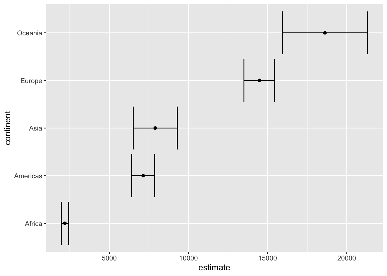
%>% group_by (continent) %>% summarise (test = list (t.test (gdpPercap))) %>% mutate (tidied = purrr:: map (test, broom:: tidy)) %>% unnest (tidied) %>% ggplot (aes (estimate, continent)) + geom_point () + geom_errorbarh (aes (xmin = conf.low,xmax = conf.high
count() + fct_reorder() + geom_col() + coord_flip()
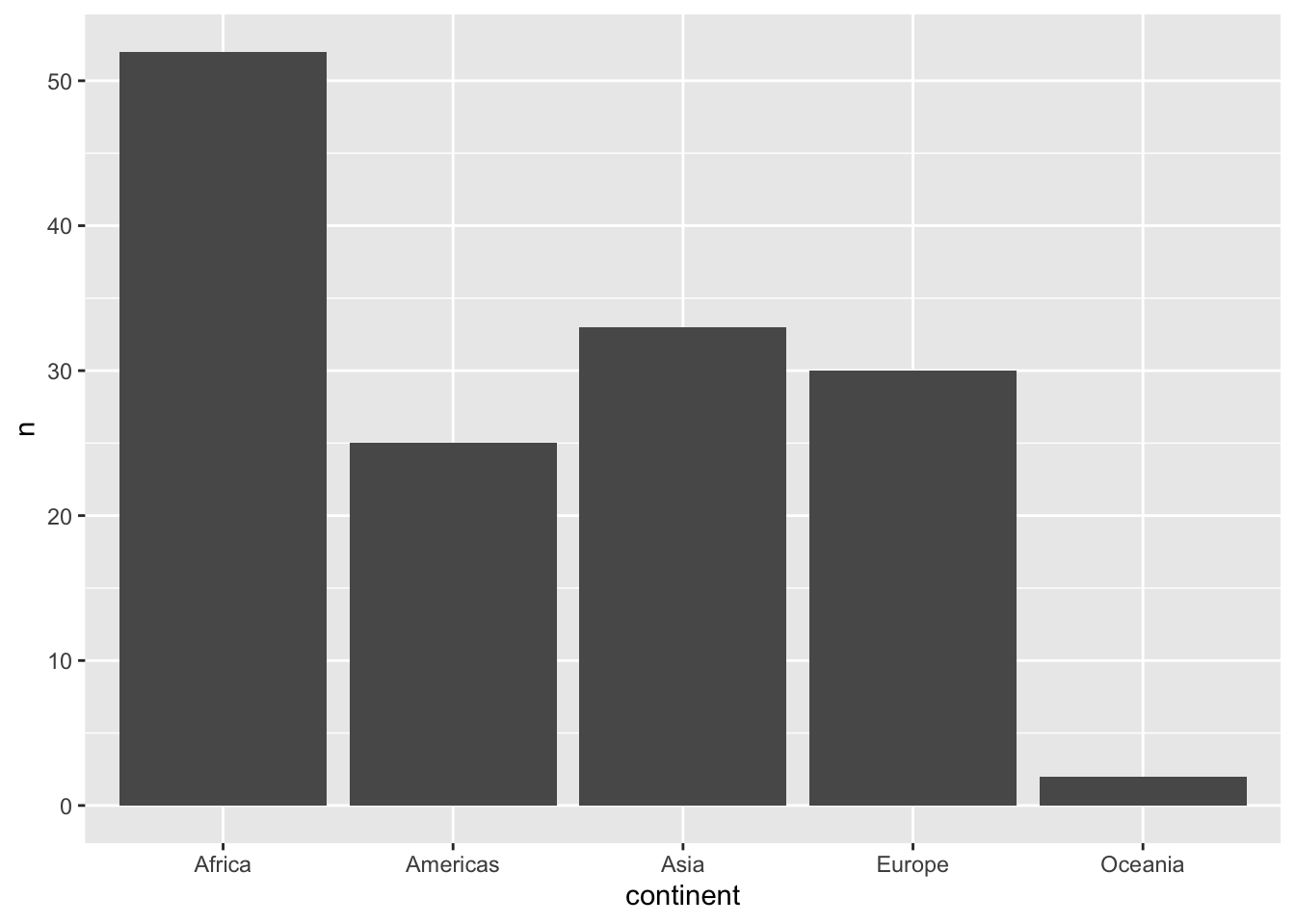
%>% distinct (continent,country)%>% count (continent)%>% ggplot (aes (x= continent,y= n))+ geom_col ()
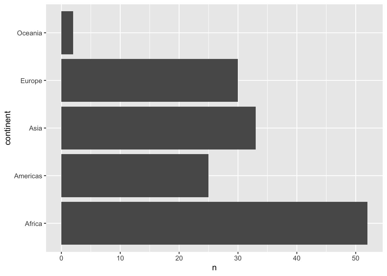
将其x转换到y轴:
%>% distinct (continent,country)%>% count (continent)%>% ggplot (aes (x= continent,y= n))+ geom_col ()+ coord_flip ()
distinct: keep only unique rows from a data frame.
%>% distinct (continent, country) %>% count (continent)
# A tibble: 5 × 2
  continent     n
  <fct>     <int>
1 Africa       52
2 Americas     25
3 Asia         33
4 Europe       30
5 Oceania       2
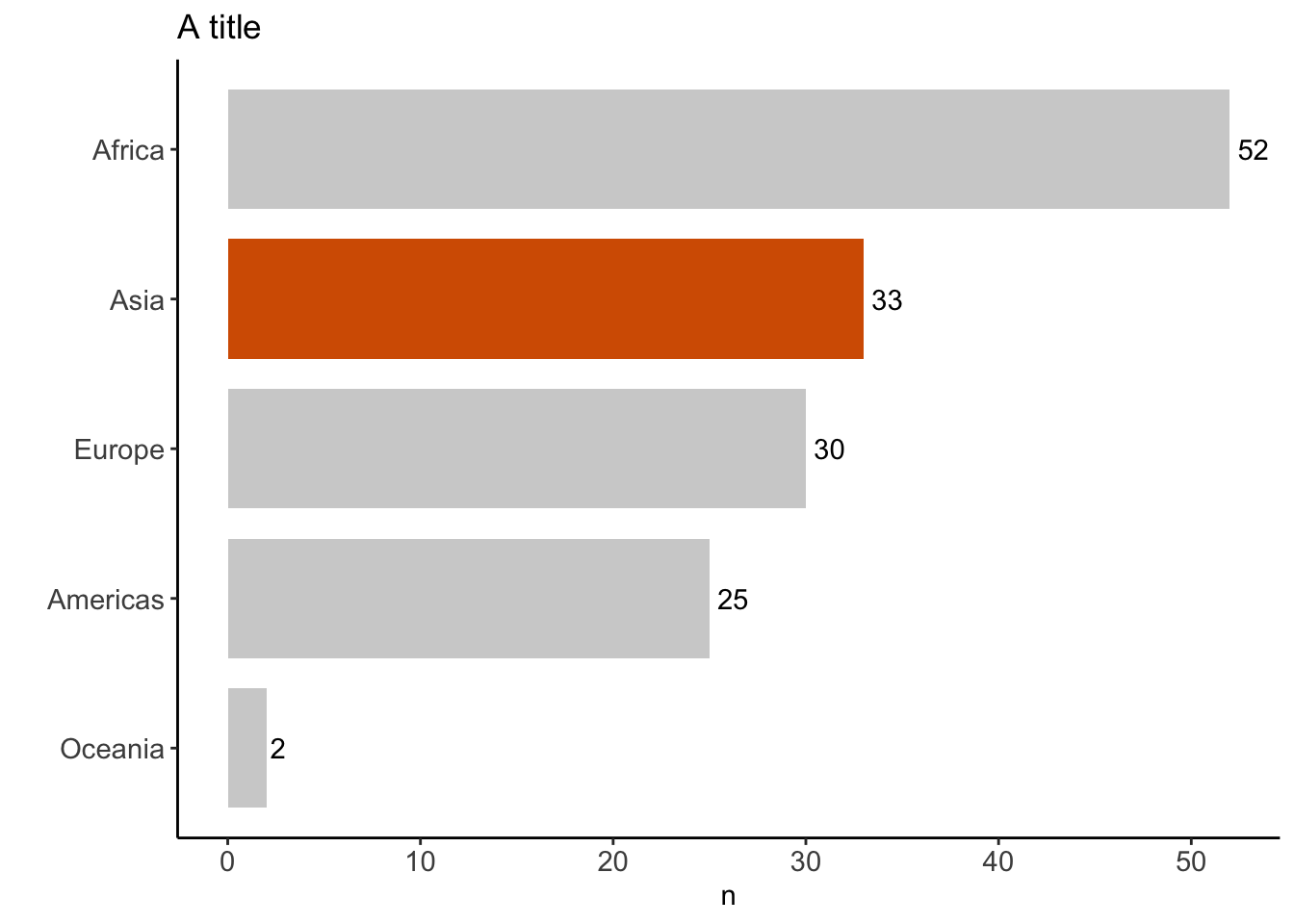
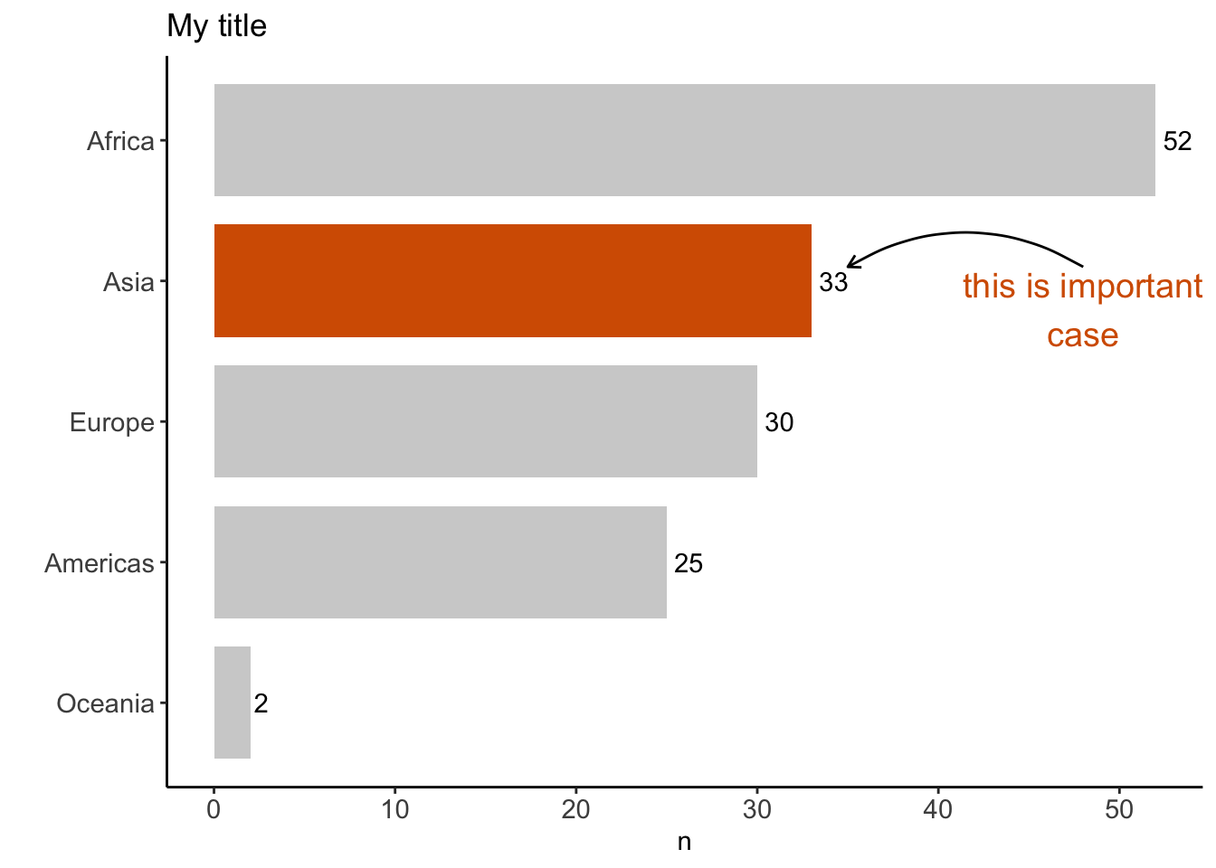
%>% distinct (continent, country) %>% count (continent)%>% mutate (coll = if_else (continent == "Asia" , "red" , "gray" )) %>% ggplot (aes (x = fct_reorder (continent, n), y = n)) + geom_text (aes (label = n), hjust = - 0.25 ) + geom_col (width = 0.8 , aes (fill = coll) ) + coord_flip () + theme_classic () + scale_fill_manual (values = c ("#b3b3b3a0" , "#D55E00" )) + theme (legend.position = "none" ,axis.text = element_text (size = 11 )+ labs (title = "A title" , x = "" )
添加annotate:
%>% distinct (continent, country) %>% count (continent) %>% ggplot (aes (x = fct_reorder (continent, n), y = n)) + geom_text (aes (label = n), hjust = - 0.25 ) + geom_col (width = 0.8 , aes (fill = continent == "Asia" ) ) + coord_flip () + theme_classic () + scale_fill_manual (values = c ("#b3b3b3a0" , "#D55E00" )) + annotate ("text" , x = 3.8 , y = 48 , label = "this is important \n case" , color = "#D55E00" , size = 5 ) + annotate (geom = "curve" , x = 4.1 , y = 48 , xend = 4.1 , yend = 35 , curvature = .3 , arrow = arrow (length = unit (2 , "mm" ))+ theme (legend.position = "none" ,axis.text = element_text (size = 11 )+ labs (title = "My title" , x = "" )
scoped()函数
对所有的列操作,使用_all;
对数据框指定的几列进行操作,可采用_at实现;
对数据框符合条件的几列进行操作,可以使用_if实现;
<- iris %>% as_tibble () <- iris %>% head (5 )
# A tibble: 5 × 5
  Sepal.Length Sepal.Width Petal.Length Petal.Width Species
         <dbl>       <dbl>        <dbl>       <dbl> <fct>
1          5.1         3.5          1.4         0.2 setosa
2          4.9         3            1.4         0.2 setosa
3          4.7         3.2          1.3         0.2 setosa
4          4.6         3.1          1.5         0.2 setosa
5          5           3.6          1.4         0.2 setosa
%>% mutate_if (is.double, as.integer)
# A tibble: 5 × 5
  Sepal.Length Sepal.Width Petal.Length Petal.Width Species
         <int>       <int>        <int>       <int> <fct>
1            5           3            1           0 setosa
2            4           3            1           0 setosa
3            4           3            1           0 setosa
4            4           3            1           0 setosa
5            5           3            1           0 setosa
也可将函数写在list()中,使用purrr-style lambda形式写出
%>% mutate_if (is.numeric, list (~ scale (.), ~ log (.)))
# A tibble: 5 × 13
Sepal.Length Sepal.W…¹ Petal…² Petal…³ Species Sepal…⁴ Sepal…⁵ Petal…⁶ Petal…⁷
<dbl> <dbl> <dbl> <dbl> <fct> <dbl> <dbl> <dbl> <dbl>
1 5.1 3.5 1.4 0.2 setosa 1.16 0.850 0 NaN
2 4.9 3 1.4 0.2 setosa 0.193 -1.08 0 NaN
3 4.7 3.2 1.3 0.2 setosa -0.772 -0.309 -1.41 NaN
4 4.6 3.1 1.5 0.2 setosa -1.25 -0.695 1.41 NaN
5 5 3.6 1.4 0.2 setosa 0.675 1.24 0 NaN
# … with 4 more variables: Sepal.Length_log <dbl>, Sepal.Width_log <dbl>,
# Petal.Length_log <dbl>, Petal.Width_log <dbl>, and abbreviated variable
# names ¹Sepal.Width, ²Petal.Length, ³Petal.Width, ⁴Sepal.Length_scale[,1],
# ⁵Sepal.Width_scale[,1], ⁶Petal.Length_scale[,1], ⁷Petal.Width_scale[,1]
我们使用slect加上_if就可以实现条件筛选变量:
<- tibble:: tibble (x = letters[1 : 3 ],y = c (1 : 3 ),z = c (0 , 0 , 0 )
# A tibble: 3 × 3
  x         y     z
  <chr> <int> <dbl>
1 a         1     0
2 b         2     0
3 c         3     0
%>% select_if (is.numeric)
# A tibble: 3 × 2
      y     z
  <int> <dbl>
1     1     0
2     2     0
3     3     0
输入的为函数,同时都是作用在列上。
filter_if()函数
进一步的,我们还有filter_if:
<- ggplot2:: msleep%>% :: select (name, sleep_total) %>% :: filter (sleep_total > 18 )
# A tibble: 4 × 2
  name                 sleep_total
  <chr>                      <dbl>
1 Big brown bat               19.7
2 Thick-tailed opposum        19.4
3 Little brown bat            19.9
4 Giant armadillo             18.1
filter_if能够帮助我们在单个数据维度上进行操作,之前的scoped函数都是在列上进行操作计算。 同时,filter_if()能够结合一些统计计算的函数,包括%in%,between()等。
%>% :: select (name, sleep_total) %>% :: filter (between (sleep_total, 16 , 18 ))
# A tibble: 4 × 2
  name                   sleep_total
  <chr>                        <dbl>
1 Owl monkey                    17
2 Long-nosed armadillo          17.4
3 North American Opossum        18
4 Arctic ground squirrel        16.6
%>% filter_all (all_vars (. > 150 ))
 [1] mpg  cyl  disp hp   drat wt   qsec vs   am   gear carb
<0 rows> (or 0-length row.names)
all_vars(.)能够用于帮助我们对所有的数据超过或不超过等条件进行筛选。any_vars()能够对所有数据凡是满足条件即保留。
group_by函数
%>% dplyr:: group_by (cyl)
# A tibble: 32 × 11
# Groups:   cyl [3]
     mpg   cyl  disp    hp  drat    wt  qsec    vs    am  gear  carb
   <dbl> <dbl> <dbl> <dbl> <dbl> <dbl> <dbl> <dbl> <dbl> <dbl> <dbl>
 1  21       6  160    110  3.9   2.62  16.5     0     1     4     4
 2  21       6  160    110  3.9   2.88  17.0     0     1     4     4
 3  22.8     4  108     93  3.85  2.32  18.6     1     1     4     1
 4  21.4     6  258    110  3.08  3.22  19.4     1     0     3     1
 5  18.7     8  360    175  3.15  3.44  17.0     0     0     3     2
 6  18.1     6  225    105  2.76  3.46  20.2     1     0     3     1
 7  14.3     8  360    245  3.21  3.57  15.8     0     0     3     4
 8  24.4     4  147.    62  3.69  3.19  20       1     0     4     2
 9  22.8     4  141.    95  3.92  3.15  22.9     1     0     4     2
10  19.2     6  168.   123  3.92  3.44  18.3     1     0     4     4
# … with 22 more rows
列名清理
数据框的列名,不要用有空格和中文。 如果拿到的原始数据中列比较多,手动修改麻烦,可以使用janitor::clean_names()函数。
library (readxl)library (janitor) # install.packages("janitor")
Attaching package: 'janitor'
The following objects are masked from 'package:stats':

    chisq.test, fisher.test
缺失值处理
library (purrr)<- as_tibble (airquality)%>% purrr:: map (~ sum (is.na (.)))
$Ozone
[1] 37

$Solar.R
[1] 7

$Wind
[1] 0

$Temp
[1] 0

$Month
[1] 0

$Day
[1] 0
%>% :: map_df (~ sum (is.na (.)))
# A tibble: 1 × 6
  Ozone Solar.R  Wind  Temp Month   Day
  <int>   <int> <int> <int> <int> <int>
1    37       7     0     0     0     0
缺失值替换
%>% mutate_all (funs (replace (., is.na (.), 0 )))
Warning: `funs()` was deprecated in dplyr 0.8.0.
ℹ Please use a list of either functions or lambdas:

# Simple named list: list(mean = mean, median = median)

# Auto named with `tibble::lst()`: tibble::lst(mean, median)

# Using lambdas list(~ mean(., trim = .2), ~ median(., na.rm = TRUE))
# A tibble: 153 × 6
   Ozone Solar.R  Wind  Temp Month   Day
   <dbl>   <dbl> <dbl> <dbl> <dbl> <dbl>
 1    41     190   7.4    67     5     1
 2    36     118   8      72     5     2
 3    12     149  12.6    74     5     3
 4    18     313  11.5    62     5     4
 5     0       0  14.3    56     5     5
 6    28       0  14.9    66     5     6
 7    23     299   8.6    65     5     7
 8    19      99  13.8    59     5     8
 9     8      19  20.1    61     5     9
10     0     194   8.6    69     5    10
# … with 143 more rows
参考资料
https://bookdown.org/wangminjie/R4DS/tidyverse-dplyr-adv.html#across%E5%87%BD%E6%95%B0-1